Understanding the Forward and Backward Pass of FlashAttention2
As compute continues to scale faster than bandwidth1, it’s important to design IO-aware algorithms that reduce memory consumption and traffic, while effectively utilizing available functional units as much as possible. This is precisely the purpose of the FlashAttention algorithms (now up to FA4!). At a high level, FlashAttention is a memory-efficient algorithm for computing the exact attention mechanism without needing to materialize large matrices in global memory and making sure the Tensor Cores on GPUs remain busy2. While I’ll focus on FA2 in this post, the lessons learned will carry over to newer versions.
For this post in particular, I’d like to build up to an understanding of the backward pass of FA2. Which tensors are being saved during the forward pass? How do these tensors help during the backward pass? What benefits does a two-pass algorithm provide us? Along the way, we will go over the forward pass, write some Triton code, and become familiar with profiling tools such as NVIDIA Nsight Systems.
I ran all experiments on a single 3090 GPU which has roughly 24 GiB of global memory and 48 KiB of shared memory per thread block. The 3090 is also equipped with Tensor Cores (although no Tensor Memory Accelerator). I’ll assume familiarity with the memory hierarchy in GPUs. As a reference, I really like the GPU Glossary from Modal: https://modal.com/gpu-glossary.
All the code for this blog post can be found at: https://github.com/kvgarimella/flashattention2-backward.
The Forward Pass
Let’s start with the forward pass. Since there are several excellent blog posts on the forward pass of FlashAttention, I’ll keep this section brief and focus on profiling. Here is the configuration I’ll use for the Nsight experiments throughout this post:
batch size: 4
hidden dimension: 64
sequence length: 8192
datatype: float32
Let’s first write out the attention forward pass. For input matrices, $\mathbf{Q}, \mathbf{K}, \mathbf{V} \in \mathbb{R}^{N \times d}$ where $N$ is the sequence length and $d$ is the hidden dimension (usually the head dimension), we compute:
\[\begin{alignedat}{2} \mathbf{S} &= \mathbf{Q} \mathbf{K}^T / \sqrt{d} &\quad&\in \mathbb{R}^{N \times N} \\ \mathbf{P} &= \mathrm{softmax}(\mathbf{S}) &\quad&\in \mathbb{R}^{N \times N} \\ \mathbf{O} &= \mathbf{P} \mathbf{V} &\quad&\in \mathbb{R}^{N \times d} \end{alignedat}\]Here, masking is applied to $\mathbf{S}$ and the softmax is per-row. As the sequence length $N$ grows, both the $\mathbf{S}$ and $\mathbf{P}$ matrices introduce major memory pressure. Below is a visualization of self-attention shown to scale:
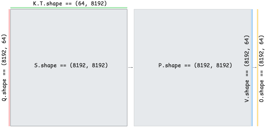
For an even larger context length of $N = 65,536$, the attention matrix $\mathbf{S}$ is 16 GiB in float32. Let’s do some profiling to gain a better understanding.
Eager Mode
We will start with a from-scratch eager implementation of the algorithm:
import math
import torch
from einops import einsum

def scaled_dot_product_attention(
    queries: torch.Tensor, # (bsz, ..., seq_len, d)
    keys: torch.Tensor,    # (bsz, ..., seq_len, d)
    values: torch.Tensor,  # (bsz, ..., seq_len, d)
    is_causal: bool = False,
) -> torch.Tensor:
    # computing attention
    scale = 1.0 / math.sqrt(queries.shape[-1])
    S = einsum(queries, keys, "... t d, ... T d -> ... t T") * scale

    # masking
    if is_causal:
        n_queries, n_keys = queries.shape[-2], keys.shape[-2]
        q_idx = torch.arange(n_queries, device=queries.device)[:, None]
        k_idx = torch.arange(n_keys, device=queries.device)[None, :]
        S = S.masked_fill(k_idx > q_idx, float("-inf"))

    # computing softmax
    P = softmax(S, dim=-1)

    # linear combination
    return einsum(P, values, "... t T, ... T d -> ... t d")

def softmax(x: torch.Tensor, dim: int) -> torch.Tensor:
    safe_x = x - torch.amax(x, dim, keepdim=True)
    exp_x = torch.exp(safe_x)
    return exp_x / torch.sum(exp_x, dim, keepdim=True)
We can profile this code using Nsight Systems, which will show us the exact CUDA kernels launched during the forward pass (blue boxes in the figure below). I used nvtx ranges to annotate sections of the code above.
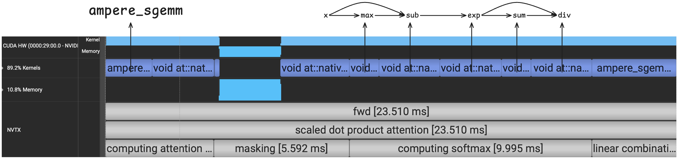
This kernel took 23.51 ms on the 3090. First, we’ll note that only the first and last kernels are GEMMs (for computing $\mathbf{S}$ and $\mathbf{O}$), and both are running on the CUDA Cores rather than the Tensor Cores (ampere_sgemm). This is because we are using float32 as the datatype. Besides the two GEMMs, the eager implementation has several element-wise and reduce kernels (these start with void at::native).
Each of the CUDA kernels moves data from global memory into the GPU’s SMs and back to global memory3. In fact, many of these kernels will move an $N \times N$ matrix to and from global memory (e.g., the exp kernel within softmax). Finally, we can see that the softmax computation consists of 5 SIMT kernels, which I’ve associated with their corresponding function calls in the code block above. The softmax computation has a relatively low arithmetic intensity and takes up more time than any other computation during the forward pass.
Compile Mode
What does torch.compile give us on the exact same code block? Let’s check the profiler output:
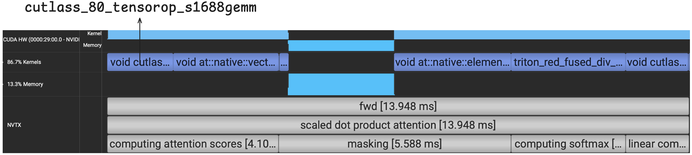
With torch.compile, the runtime is now reduced to 13.95 ms. We can see that the GEMMs for computing $\mathbf{S}$ and $\mathbf{O}$ are now running on the Tensor Cores as opposed to the CUDA Cores using the TF32 datatype (cutlass_80_tensorop_s1688gemm).
For computing $\mathbf{S}$ (which requires a GEMM and an element-wise kernel), more time is now spent on the element-wise multiply with the scaling factor rather than the GEMM itself. We are paying the price of bringing a large matrix on-chip just to perform a simple multiply and sending it right back to global memory.
For softmax, we can see that the entire calculation has now been fused into a single kernel (starting with triton_red_fused). Even so, this compiled run still requires storing the $N \times N$ matrices $\mathbf{S}$ and $\mathbf{P}$ to global memory. To visualize this, let’s plot the memory usage after the forward pass for eager, compile, and an implementation of FA2 in Triton.
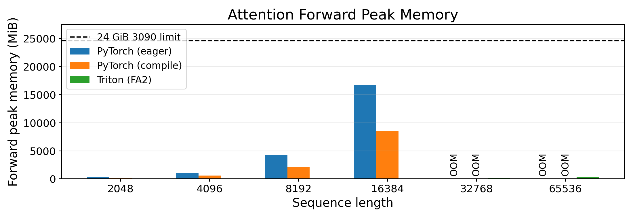
With torch.compile, we’ve at least reduced memory usage since many ops have been fused (fewer intermediate activations are stored) and we’ve reduced memory traffic since there are fewer CUDA kernel launches. Still, the compiled version OOMs on the 3090 for a sequence length of $N = 32768$. In other words, even with torch.compile, we haven’t “re-discovered” the FlashAttention algorithm itself. On the other hand, FlashAttention2’s memory usage is hardly visible on the graph!
Let’s now implement the forward pass of FA2 to understand how we can bypass this memory issue and to set ourselves up for understanding the backward pass.
FlashAttention2 with Triton
If we treat the scaled_dot_product_attention function in the code block above as a black box, all we really care about is taking as input three matrices $\mathbf{Q}$, $\mathbf{K}$, and $\mathbf{V}$ of size $N \times d$ and producing an output matrix $\mathbf{O}$ of size $N \times d$. By viewing this function purely as an interface, there is no notion of the large matrices $\mathbf{S}$ and $\mathbf{P}$.
This is exactly what FlashAttention2 does. It is an implementation of the attention layer that, through tiling and the online softmax trick4, does not need to create or store any large intermediate matrices but still produces the desired result. The high-level idea is to compute a tile of the output matrix $\mathbf{O}$ from tiles of the input matrices $\mathbf{Q}$, $\mathbf{K}$, and $\mathbf{V}$. The intermediate per-row softmax operation can then be directly baked into this tiled computation.
Before showing the full algorithm, let’s first go over the online softmax trick since that will make the forward pass easier to understand. Remember that for a particular row $s \in \mathbb{R}^{N}$ of the matrix $\mathbf{S}$, we would like to obtain $\mathrm{softmax}(s)_i = \frac{\exp{(s_i - \max(s))}}{\sum_j \exp{(s_j - \max(s))}}$ where $\max(s)$ is the maximum value in the vector $s$.
The online softmax trick is a way to obtain both the maximum and the denominator (the sum) in a single pass over the vector. As we iterate over the vector values, it’s straightforward to obtain the maximum; just keep a running maximum. Since the denominator depends upon the final maximum value, how do we obtain the correct sum during this single pass? The key is to introduce a correction term (I’ll call it rescale in the code block below) that can be used to update previously summed values. The code block below shows this trick:
import torch
torch.manual_seed(42)

vals = torch.randn(8)
softmax_ref = torch.softmax(vals, dim=0)

# Online version
# Assume we are streaming in the row one value at a time
BLOCK = 1 # a "block" is just one value
running_max = torch.tensor(float('-inf'))
running_sum = torch.tensor(0.0)
for i in range(0, len(vals), BLOCK):
    block = vals[i:i + BLOCK]
    block_max = torch.max(block)

    new_max = torch.max(running_max, block_max)
    rescale = torch.exp(running_max - new_max) # correction term for the old running sum
    running_sum = rescale * running_sum + torch.sum(torch.exp(block - new_max))
    running_max = new_max

softmax_online = torch.exp(vals - running_max) / running_sum
print(torch.allclose(softmax_ref, softmax_online))
As an example, suppose we want to calculate the denominator of softmax for the vector [0.5, 2.0, 1.0]. Since the maximum is 2.0, we should get: exp(0.5 - 2.0) + exp(2.0 - 2.0) + exp(1.0 - 2.0). The online algorithm above will calculate this as: exp(0.5 - 2.0) * exp(0.5 - 0.5) + exp(2.0 - 2.0) + exp(1.0 - 2.0). The running sum after the first iteration was exp(0.5 - 0.5) but the rescale value during the second iteration corrects this term. The rescale term during the third and final iteration is just 1.0 since the running maximum has not changed.
This exact rescale term will be used in the FlashAttention algorithm to correct both the running sum for each row of $\mathbf{S}$ and the running calculation of a tile of $\mathbf{O}$. Instead of streaming one value at a time, FlashAttention streams in tiles and the same online trick will still work. You can verify this by changing BLOCK = 2 above.
Now that we are equipped with the online softmax trick, let’s look at the forward pass of FlashAttention using a figure and some pseudo-code.
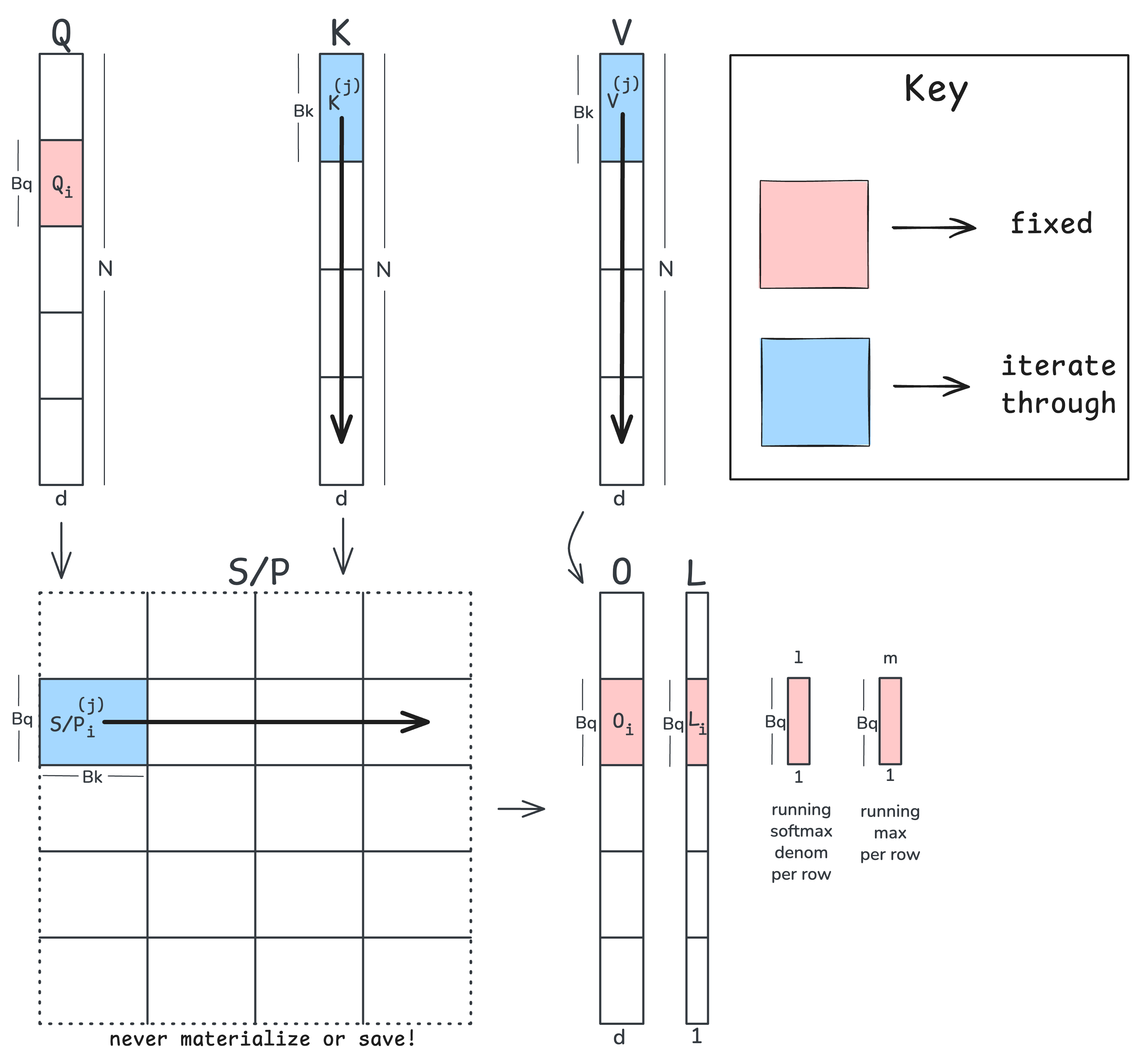
At a high level, we will fix a tile of $\mathbf{Q}$ and iterate over tiles of $\mathbf{K}$ and $\mathbf{V}$ to calculate a fixed tile of the output matrix $\mathbf{O}$. We will also keep a running denominator and maximum term (shown in the figure as l and m) as we iterate over tiles of $\mathbf{K}$/$\mathbf{V}$. At the end, we combine l and m to store the logsumexp of the attention scores ($L$ in the figure). We will see how storing $L$ makes for a more efficient backward pass. Here is the pseudo-code:
Load into SRAM Q_i    ∈ R^(B_q × d) # a tile of the query matrix Q
Init in SRAM O_i ← 0  ∈ R^(B_q × d) # a tile of the output matrix O
Init in SRAM L_i ← 0  ∈ R^(B_q × 1) # a tile of the logsumexp L
Init in SRAM ℓ ← 0    ∈ R^(B_q × 1) # running sum (denominator: sum of exps)
Init in SRAM m ← -∞   ∈ R^(B_q × 1) # running max

T_c = ⌈N / B_k⌉ # number of K/V tiles
for j = 1 to T_c:
    # 1. Load K/V tiles
    load into SRAM K_j, V_j # (B_k × d)

    # 2. Compute an attention tile
    S ← Q_i @ K_jᵀ # (B_q × d) @ (d × B_k) = (B_q × B_k)

    # 3. Online softmax update
    m_new   ← max(m, rowmax(S)) # (B_q × 1), (B_q × 1) = (B_q × 1)
    rescale ← exp(m - m_new)    # (B_q × 1) - (B_q × 1) = (B_q × 1)

    # 4. numerator of softmax for current tile
    P ← exp(S - m_new) # (B_q × B_k) - (B_q × 1) = (B_q × B_k)

    # 5. Rescale old running sum and O tile and add current tile values
    ℓ   ← rescale * ℓ + rowsum(P) # (B_q × 1) * (B_q × 1) + (B_q × 1) = (B_q × 1)
    O_i ← rescale * O_i + P @ V_j # (B_q × 1) * (B_q × d) + (B_q × d) = (B_q × d)

    # 6. Update the running maximum
    m ← m_new # (B_q × 1)

# 7. Divide by running sum and store
O_i ← O_i / ℓ # (B_q × d) / (B_q × 1)
Store O_i in global memory

# 8. Store logsumexp of attention scores for use during backward pass
L_i ← m + log(ℓ)  # (B_q × 1) + (B_q × 1) = (B_q × 1)
Store L_i in global memory
This algorithm is similar to the tiled online softmax trick but folds in both matrix multiplies in the attention mechanism. Let’s walk through each step:
- Load in a tile of $\mathbf{K}$ and $\mathbf{V}$. Remember that the tiles of $\mathbf{Q}$ and $\mathbf{O}$ are fixed.
- Calculate a tile of the matrix $\mathbf{S}$. Nothing too fancy here, we are just tiling up our $\mathbf{Q}$ and $\mathbf{K}$ matrices and performing a tile-sized matmul.
- The online softmax max and rescale calculation, except that we are working with vectors of size $B_q \times 1$. All computations are independent, row-wise given that softmax operates over rows of $\mathbf{S}$.
- We perform the numerator of the safe softmax for $\mathbf{S}$ with the latest maximum we’ve seen per row.
- Our rescale trick for the running sum is the same as before except we are working on vectors of size $B_q \times 1$. The same rescale trick works for our running calculation of the $\mathbf{O}$ tile since
P @ Vis linear. - Update the running maximum per row.
- Normalize the tile of $\mathbf{O}$ by the running sum and store to global memory
- Store the corresponding tile of the logsumexp, $L$.
We can perform these steps for each sample, head, and each tile of $\mathbf{Q}$ and $\mathbf{O}$ in parallel. Therefore in Triton, we launch batch_size x number of heads x number Q/O tiles programs in parallel. Importantly, we never have to materialize or store the full $N \times N$ attention matrices $\mathbf{S}$ and $\mathbf{P}$ and yet will still arrive at the correct output matrix $\mathbf{O}$! Note that due to linearity, we can divide the output by the normalization terms after multiplying by the matrix $\mathbf{V}$.
We will be using Triton to implement this algorithm since its programming model allows one to operate at the tile level and explicitly load/store data from on-chip shared memory. There are plenty of other languages too at roughly the same abstraction level, for example cuTile or Pallas.
Rather than dump the code in this post, I’ll just link to it here starting at the for loop over the $\mathbf{K}$/$\mathbf{V}$ tiles. We do a couple of extra things like causal masking and skipping tiles in which all key indices are greater than the query indices (i.e., tiles that are entirely above the causal diagonal).
In the Triton code itself, look out for the use of tl.dot which performs the tile-sized matmuls on the Tensor Cores. We can verify the use of Tensor Cores by checking the output PTX from our Triton kernel, and we will see several instances of mma.sync.aligned.m16n8k8.row.col.f32.tf32.tf32.f32.
What does the corresponding Nsight output look like?

Unsurprisingly, there is just a single kernel launch, and we’ve now reduced the runtime to just 2.19 ms. This speedup comes from several optimizations: one kernel launch, Tensor Cores GEMMs, and we don’t repeatedly read and write $\mathbf{S}$/$\mathbf{P}$ from global memory. We have also reduced the memory usage from many GiBs to a few MiBs by not storing $\mathbf{S}$ or $\mathbf{P}$ to global memory.
Summarizing the forward pass, we’ve gone from (eager) 23.51 ms $\rightarrow$ (torch.compile) 13.95 ms $\rightarrow$ (Triton) 2.19 ms while greatly reducing the memory pressure from O(GiB) $\rightarrow$ O(MiB). Let’s now turn to the backward pass and see how we utilize the logsumexp, $L$ we stored during the forward pass. We will also see how performing more compute can save time by avoiding atomic adds.
The Backward Pass
Suppose now we are doing a backward pass and have $\partial\mathsf{loss}/\partial\mathbf{O}$ (which we write as just $\mathbf{dO}$). Our goal is to calculate $\mathbf{dQ}$, $\mathbf{dK}$, and $\mathbf{dV}$ from $\mathbf{dO}$ all of which have shape $N \times d$. Similar to the forward pass, we can obtain these gradients without materializing the full $N \times N$ matrices such as $\mathbf{P}$, $\mathbf{dP}$, and $\mathbf{dS}$. We will see that there are two auxiliary tensors ($L$ and $D$) that allow us to efficiently perform back propagation.
Let’s first re-write the forward pass:
\[\mathbf{S} = \mathbf{Q}\mathbf{K}^T / \sqrt{d}, \quad \mathbf{P} = \mathrm{softmax}(\mathbf{S}), \quad \mathbf{O} = \mathbf{P}\mathbf{V}\]And the backward pass:
\[\begin{alignedat}{2} \mathbf{dV} &= \mathbf{P}^T\mathbf{dO} &\quad&\in \mathbb{R}^{N \times d} \\ \mathbf{dP} &= \mathbf{dO}\mathbf{V}^T &\quad&\in \mathbb{R}^{N \times N} \\ \mathbf{dS} &= \mathsf{dsoftmax}(\mathbf{P}, \mathbf{dP}) &\quad&\in \mathbb{R}^{N \times N} \\ \mathbf{dQ} &= \mathbf{dS}\mathbf{K} / \sqrt{d} &\quad&\in \mathbb{R}^{N \times d} \\ \mathbf{dK} &= \mathbf{dS}^T \mathbf{Q} / \sqrt{d} &\quad&\in \mathbb{R}^{N \times d} \\ \end{alignedat}\]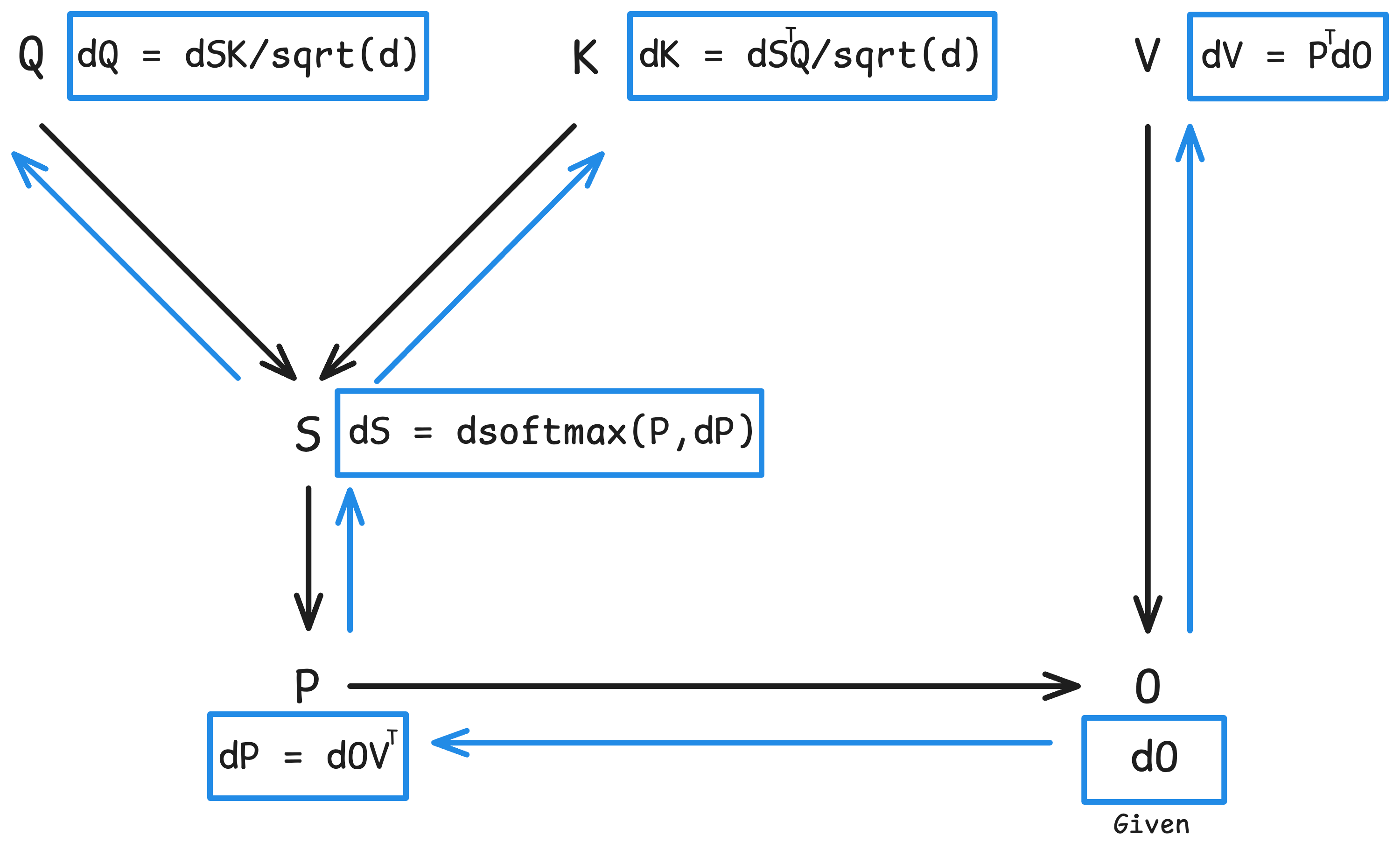
Again, both $\mathbf{P}$ during the forward and $\mathbf{dS}$ during the backward pass are row-wise independent. Let’s now define $\mathbf{dS}$. To simplify, suppose we take a look at one row of $\mathbf{S}$, which I’ll call $\mathbf{S}_i \in \mathbb{R}^{1 \times N}$. We have:
\[\begin{aligned} \mathbf{S}_i &= \left[\mathbf{S}_{i0}, \mathbf{S}_{i1}, \ldots, \mathbf{S}_{i,N - 1}\right] \\ \mathbf{P}_i &= \left[ \frac{\exp(\mathbf{S}_{i0} - m_i)}{\sum_k \exp(\mathbf{S}_{ik} - m_i)}, \cdots, \frac{\exp(\mathbf{S}_{i,N - 1} - m_i)}{\sum_k \exp(\mathbf{S}_{ik} - m_i)} \right]. \end{aligned}\]where $m_i = \max_k \mathbf{S}_{ik}$. Working through the derivative, we will see that:
\[\frac{\partial \mathbf{P}_{ij}}{\partial \mathbf{S}_{ik}} = \left\{ \begin{array}{ll} \mathbf{P}_{ij} - \mathbf{P}_{ij}\mathbf{P}_{ij}, & j = k, \\ -\mathbf{P}_{ij}\mathbf{P}_{ik}, & j \ne k. \end{array} \right\}\]We can now write the Jacobian and the gradient of a single row of $\mathbf{S}$ (remember that $\partial\mathsf{loss}/\partial\mathbf{S}_i = \mathbf{dS}_i$ ):
\[\begin{aligned} \frac{\partial \mathbf{P}_i}{\partial \mathbf{S}_i} &= \operatorname{diag}(\mathbf{P}_i) - \mathbf{P}_i^\top \mathbf{P}_i, \\ \mathbf{dS}_i &= \mathbf{dP}_i \left(\operatorname{diag}(\mathbf{P}_i) - \mathbf{P}_i^\top \mathbf{P}_i\right). \end{aligned}\]Note that both $\operatorname{diag}(\mathbf{P}_i)$ and $\mathbf{P}_i^\top \mathbf{P}_i$ are $N \times N$ matrices and we are just computing a single row of the gradient of $\mathbf{S}$.
There are two important points to make about the backward pass as we’ve written it above. First, the gradient $\mathbf{dV}$ depends upon $\mathbf{P}$ so we need to recompute (tiles of) $\mathbf{P}$ in the backward pass. We will soon see how to efficiently compute tiles of $\mathbf{P}$ without using the online softmax trick. Second, $\mathbf{dQ}$ and $\mathbf{dK}$ depend upon $\mathbf{dS}$, so we need an efficient method for obtaining $\mathbf{dS}$. As it is currently written, each row of $\mathbf{dS}$ itself depends upon an entire row of $\mathbf{P}$ rather than just a tile of $\mathbf{P}$ and computes large Jacobian matrices. Let’s now tackle both of these issues.
Recomputing $\mathbf{P}$ in the backward pass via $L$
In addition to computing $\mathbf{O}$ during the forward pass, we also computed and saved $ L \in \mathbb{R}^{N \times 1} $ which was the logsumexp of the attention matrix (step 8 in the forward pass). For a particular entry $i$ of $L$, we have
\[L_i = m_i + \log l_i = m_i + \log \sum_{k}\exp(\mathbf{S}_{ik} - m_i)\]where $m_i$ is maximum value of the $i$-th row of $\mathbf{S}$ and $l_i$ is the softmax denominator for the same row. Let’s see how this auxiliary tensor can be used during the backward pass to circumvent the online softmax trick. First, let’s write out an entry of $\mathbf{P}$:
\[\mathbf{P}_{ij} = \frac{\exp(\mathbf{S}_{ij} - m_i)}{\sum_{k}\exp(\mathbf{S}_{ik} - m_i)}\]We can re-write this expression in terms of $L_i$.
\[\begin{aligned} \mathbf{P}_{ij} &= \frac{\exp(\mathbf{S}_{ij} - m_i)} {\sum_{k}\exp(\mathbf{S}_{ik} - m_i)} \\ &= \frac{\exp(\mathbf{S}_{ij} - m_i)} {\exp\left(\log\sum_{k}\exp(\mathbf{S}_{ik} - m_i)\right)} \\ &= \frac{\exp(\mathbf{S}_{ij})} {\exp\left(m_i + \log\sum_{k}\exp(\mathbf{S}_{ik} - m_i)\right)} \\ &= \frac{\exp(\mathbf{S}_{ij})}{\exp(L_i)} \\ &= \exp(\mathbf{S}_{ij} - L_i). \end{aligned}\]Using the above expression, we can now recompute an exact tile of $\mathbf{P}$ during the backward pass without any online or running max tricks. Let’s now look at how to obtain an exact tile of $\mathbf{dS}$.
Computing $\mathbf{dS}$ from $D = \mathsf{rowsum}(O \odot dO)$
We start with our per-row gradient and then distribute the upstream gradient and group terms:
\[\begin{aligned} \mathbf{dS}_i &= \mathbf{dP}_i \left(\operatorname{diag}(\mathbf{P}_i) - \mathbf{P}_i^\top \mathbf{P}_i\right) \\ &= \mathbf{dP}_i \operatorname{diag}(\mathbf{P}_i) - \left(\mathbf{dP}_i \mathbf{P}_i^\top\right) \mathbf{P}_i. \end{aligned}\]First, since $ \operatorname{diag}(\mathbf{P}_i) $ has only one non-zero diagonal (the main diagonal), we can rewrite the first term in the above expression as element-wise multiply. Second, note that the grouping in the second term is an inner product so the output is just a single scalar value. We can write this term also as an element-wise multiply.
\[\mathbf{dS}_i = \mathbf{dP}_i \odot \mathbf{P}_i - \operatorname{sum}(\mathbf{dP}_i \odot \mathbf{P}_i) \odot \mathbf{P}_i\]Finally, we can extend down and write the full expression for $\mathbf{dS}$:
\[\mathbf{dS} = \mathbf{dP} \odot \mathbf{P} - \operatorname{rowsum}(\mathbf{dP} \odot \mathbf{P}) \odot \mathbf{P}\]Here, $\operatorname{rowsum}$ returns a column vector, which is broadcast across the columns before multiplying by $\mathbf{P}$.
Note that the above equation only uses element-wise multiplies. This is great for us since we can compute $\mathbf{dS}$ block-wise. Unfortunately, the second term requires summing over an entire row of $\mathbf{P}$. However, there is a clever substitution. First, note that $ \operatorname{rowsum}(\mathbf{dP} \odot \mathbf{P}) = \operatorname{diag}(\mathbf{dP} \mathbf{P}^\top)$. Here, $\operatorname{diag}$ is plucking out the main diagonal of an $N \times N$ matrix. Since $\mathbf{dP} = \mathbf{dO} \mathbf{V}^\top$, we can substitute and simplify $\operatorname{diag}(\mathbf{dP} \mathbf{P}^\top) = \operatorname{diag}(\mathbf{dO} \mathbf{V}^\top \mathbf{P}^\top) = \operatorname{diag}(\mathbf{dO} \mathbf{O}^T) = \operatorname{rowsum}(\mathbf{dO} \odot \mathbf{O})$. Note that both $\mathbf{dO}$ and $\mathbf{O}$ are $N \times d$, so we are now summing each row over a much smaller matrix than the $N \times N$ attention matrix $\mathbf{P}$.
Finally, putting this all together and defining $D = \operatorname{rowsum}(\mathbf{dO} \odot \mathbf{O})$, we arrive at:
\[\mathbf{dS} = \mathbf{dP} \odot \mathbf{P} - D \odot \mathbf{P} = (\mathbf{dP} - D) \odot \mathbf{P}\]Here is a “proof by code” that shows you the step by step transformation.
import math
import torch
torch.manual_seed(42)


N_q = 5; N_k = 4; d = 8
Q = torch.randn(N_q, d, requires_grad=True)
K = torch.randn(N_k, d, requires_grad=True)
V = torch.randn(N_k, d, requires_grad=True)

# Torch Backprop
S = Q @ K.T / math.sqrt(d); S.retain_grad()
P = torch.nn.functional.softmax(S, dim=-1); P.retain_grad()
O = P @ V; O.retain_grad()
L = (O**2).mean() # dummy loss func.
L.backward()

# manual backprop for dL/dS
dS = torch.empty_like(S)

# one row at a time, full Jacobian
# (1, N_k) = (1, N_k) @ (N_k, N_k)
for i in range(N_q):
    dS[i:i+1] = P.grad[i:i+1] @ (torch.diag(P[i]) - torch.outer(P[i], P[i]))
assert torch.allclose(S.grad, dS)

# one row at a time, no full Jacobian
# (N_k) = (N_k) - scalar
for i in range(N_q):
    dS[i] = (P[i] * P.grad[i] - P[i] * torch.dot(P[i], P.grad[i]))
assert torch.allclose(S.grad, dS)

# all rows at once using P and dP:
# (N_q, N_k) - (N_q, N_k) * (N_q, 1)
dS = P * P.grad - P * torch.sum(P * P.grad, dim=-1, keepdim=True)
assert torch.allclose(S.grad, dS)

# all rows at once using O and dO:
# (N_q, N_k) - (N_q, N_k) * (N_q, 1)
dS = P * P.grad - P * torch.sum(O * O.grad, dim=-1, keepdim=True)
assert torch.allclose(S.grad, dS)
Again, I’m using cross-attention ($N_q$ and $N_k$) in the code above so that tensor shapes are easier to discern. Crucially, we can now calculate $\mathbf{dS}$ without needing to sum over an entire row of $\mathbf{P} \odot \mathbf{dP}$!
Single-Pass BackProp with Atomic Adds in Triton
With the backprop math nailed down in the previous section, we can now map the backward pass to a Triton kernel. Similar to forward pass, I’ll illustrate this using a figure:
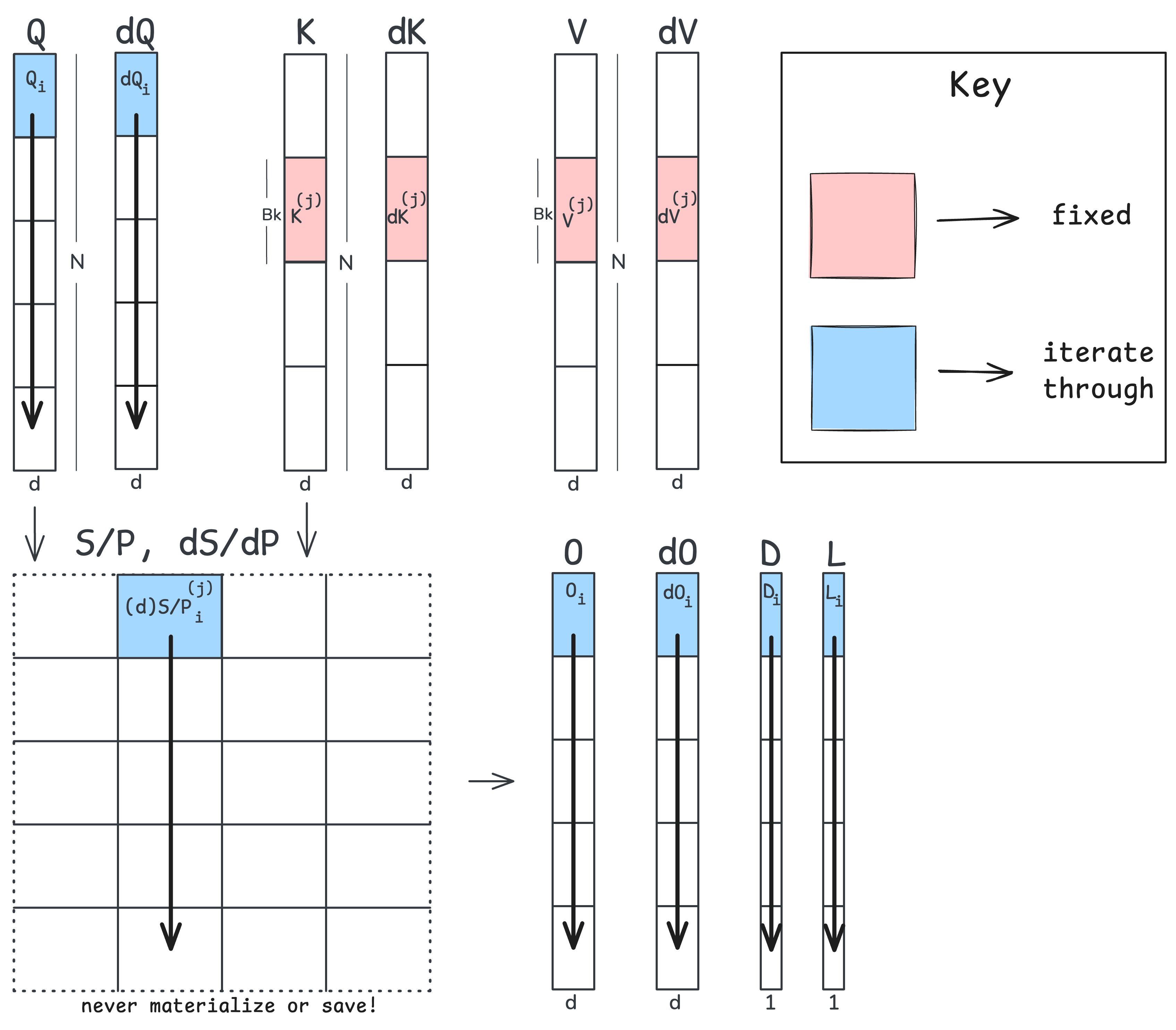
I’ll assume that we obtain $D$ a priori, although it may be calculated within the kernel as well. In contrast to the forward pass, we are now iterating down tiles of $\mathbf{Q}$ for a fixed $\mathbf{K}$/$\mathbf{V}$ tile. We do this because both $\mathbf{dK}$ and $\mathbf{dV}$ depend upon the transpose of $\mathbf{dS}$ and $\mathbf{P}$, respectively. For this reason, we can fix a tile of both $\mathbf{dK}$ and $\mathbf{dV}$ and iterate down the columns of $\mathbf{dS}$ and $\mathbf{P}$. Doing so allows us to accumulate and obtain the gradient for our fixed $\mathbf{dK}$ and $\mathbf{dV}$ tiles.
Let’s now take a look at the pseudo-code (the Triton kernel can be found here). We will recompute the forward pass up to $\mathbf{P}$ and then kick off our backpropagation up to our inputs. In the pseudo-code, pay special attention to how we update a tile of $\mathbf{dQ}$.
Load into SRAM K_j     ∈ R^(B_k × d) # a tile of the key matrix K
Load into SRAM V_j     ∈ R^(B_k × d) # a tile of the value matrix V
Init in SRAM dK_j ← 0  ∈ R^(B_k × d) # a tile of the gradient dK
Init in SRAM dV_j ← 0  ∈ R^(B_k × d) # a tile of the gradient dV

T_r = ⌈N / B_q⌉ # number of Q/O/dO tiles
for i = 1 to T_r:
    # 1. Load Q/O/dO tiles and the logsumexp from forward
    load into SRAM Q_i, O_i, dO_i # (B_q × d)
    load into SRAM L_i            # (B_q × 1)
    load into SRAM D_i            # (B_q × 1)

    # 2. Recompute an attention tile and its softmax numerator
    S ← Q_i @ K_jᵀ / sqrt(d) # (B_q × d) @ (d × B_k) = (B_q × B_k)
    P ← exp(S - L_i)         # (B_q × B_k) - (B_q × 1) = (B_q × B_k)

    # 3. Compute the local gradients through O = P @ V
    dV_j ← dV_j + Pᵀ @ dO_i # (B_k × B_q) @ (B_q × d) = (B_k × d)
    dP   ← dO_i @ V_jᵀ      # (B_q × d) @ (d × B_k) = (B_q × B_k)

    # 4. Backprop through the softmax
    dS  ← P * (dP - D_i)    # (B_q × B_k) * ((B_q × B_k) - (B_q × 1)) = (B_q × B_k)

    # 5. With dS, we can now get our gradients for K
    dK_j ← dK_j + dSᵀ @ Q_i / sqrt(d) # (B_k × B_q) @ (B_q × d) = (B_k × d)

    # 6. Atomic Add for Q (all j threads must update the same dQ_i!)
    partial_dQ_i ← dS @ K_j / sqrt(d) # (B_q × B_k) @ (B_k × d) = (B_q × d)
    atomic_add(dQ_i, partial_dQ_i)


# 7. Store dK and dV tiles in global memory
Store dK_j in global memory
Store dV_j in global memory
We’ve now obtained $\mathbf{dQ}$, $\mathbf{dK}$, and $\mathbf{dV}$ without needing to store any large $N \times N$ matrices during the forward pass and we’ve reduced forward and backward to just a single kernel launch each! Before I show the Nsight figure or talk about latencies, let’s take a look at why this single-kernel backward pass required atomic adds for $\mathbf{dQ}$.
The gradient $\mathbf{dQ}$, unlike $\mathbf{dK}$, depends upon $\mathbf{dS}$ rather than $\mathbf{dS}^T$. This means that for a fixed tile of $\mathbf{dQ}$, we’d have to march across the rows of $\mathbf{dS}$ to accumulate the gradient. This difference in dependence is exactly why our single-pass backward pass requires an atomic add for a tile of $\mathbf{Q}$. The figure below illustrates this contention:
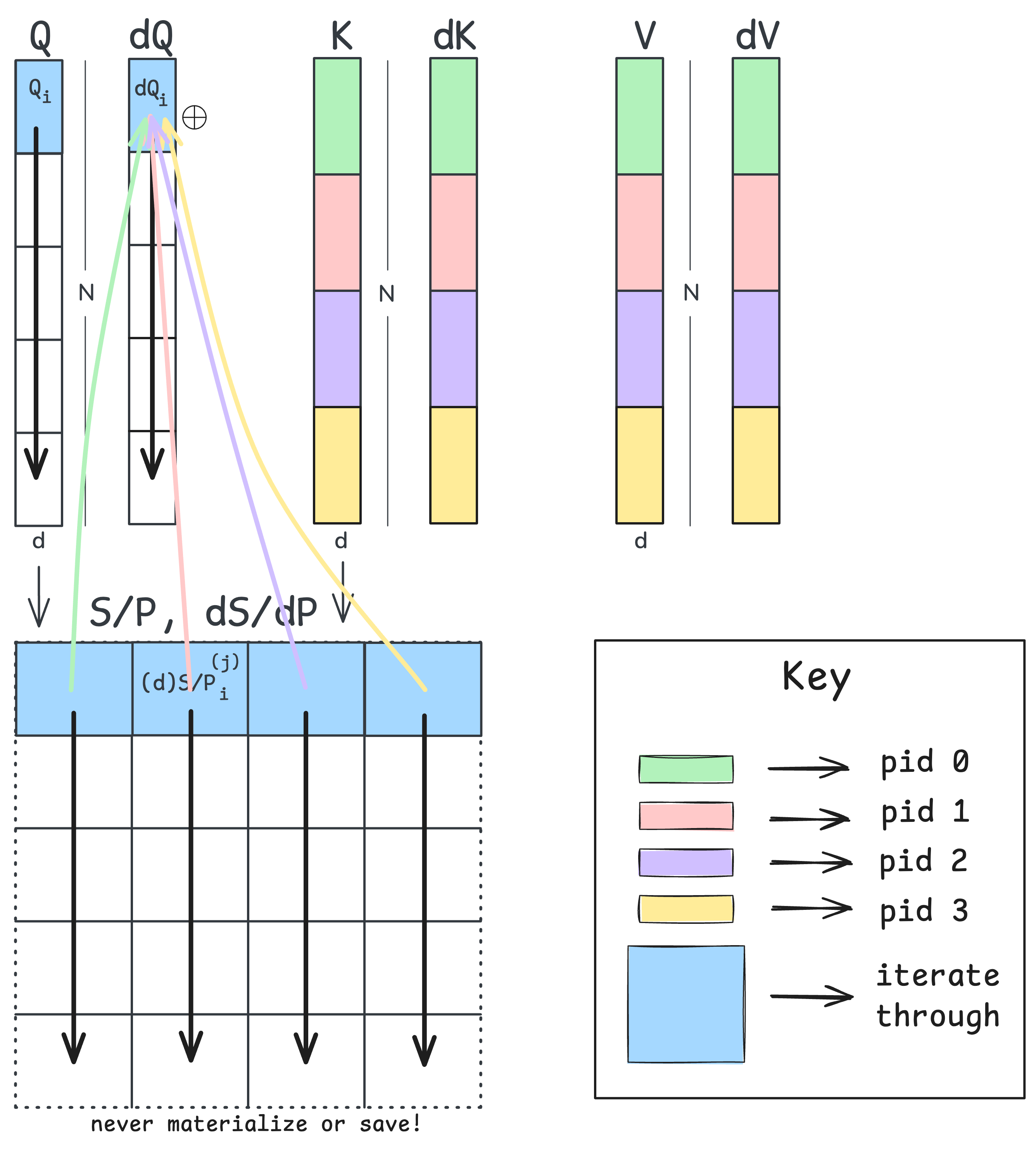
Each program instance (each separate tile of $\mathbf{K}$/$\mathbf{V}$ shown green, red, purple, and yellow) kicks off an iteration down their respective column of $\mathbf{dS}$. Each program instance must then update the same tile of $\mathbf{Q}$ before moving on to the next row. Since more than one thread is fighting to update the same tile, we need to use atomic adds to avoid race conditions.
If we were to swap the ordering and march down tiles of $\mathbf{K}$/$\mathbf{V}$ like we did in the forward pass, we would shift to two atomic adds, one for $\mathbf{dK}$ and one for $\mathbf{dV}$. For this reason, we will take a two-pass approach; one pass will be used to obtain $\mathbf{dQ}$, while the other pass calculates $\mathbf{dK}$ and $\mathbf{dV}$.
Two-Pass BackProp in Triton
The two-kernel approach removes the need for atomic adds by performing a pass across the rows of $\mathbf{S}$ and a pass down the columns of $\mathbf{S}$. The following figure illustrates this two-pass approach:
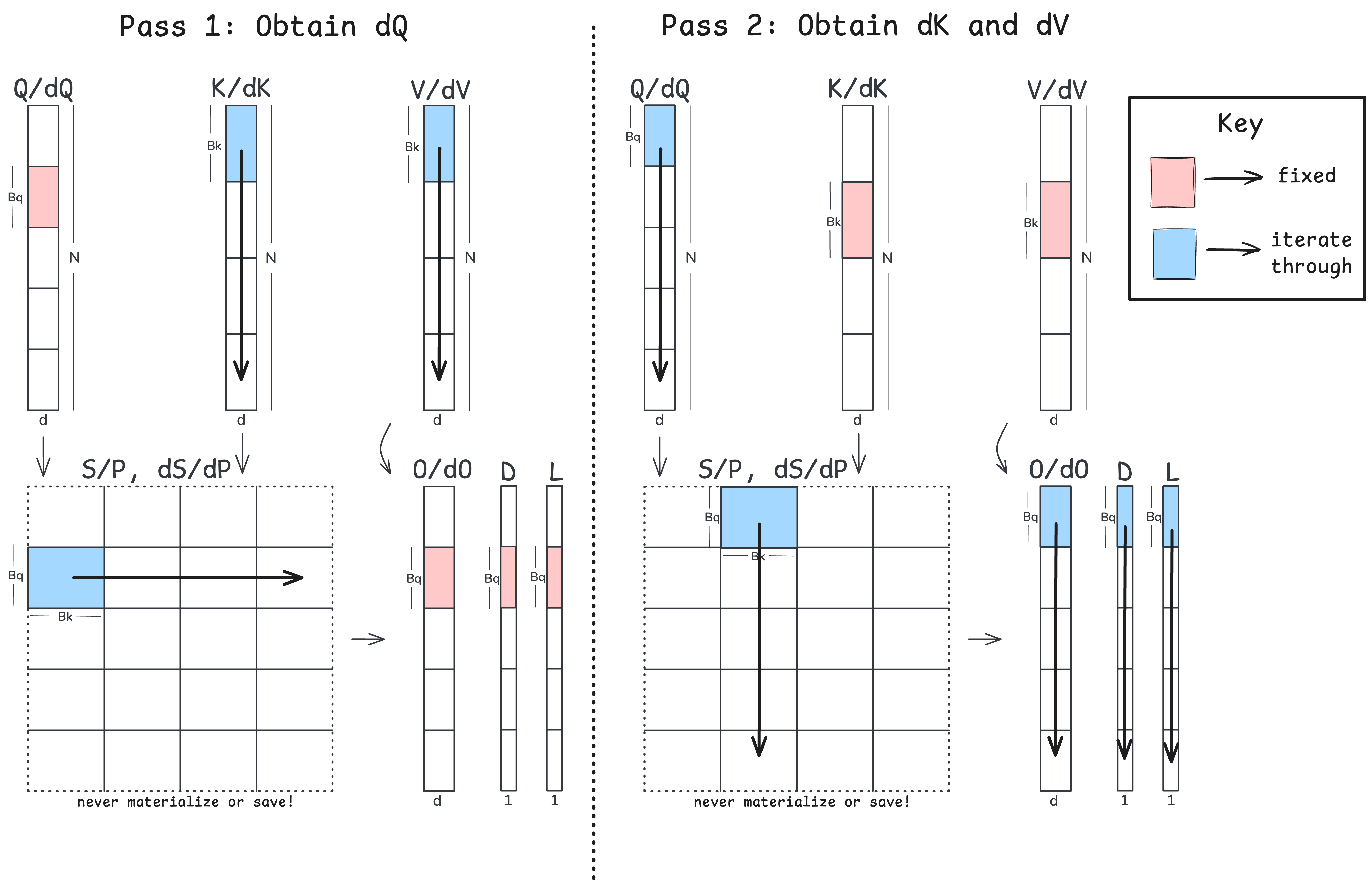
Now that we understand the mechanics of the backward pass, I’ll keep the pseudo-code here a bit high-level. You can also check out the code which has two jitted Triton kernels.
T_c = ⌈N / B_k⌉ # number of K/V tiles
for j = 1 to T_c:
    - forward pass to P
    - backward pass up to dQ

T_r = ⌈N / B_q⌉ # number of Q tiles
for i = 1 to T_r:
    - forward pass to P
    - backward pass up to dK and dV
Note that with the two-pass algorithm, we are recomputing $\mathbf{S}$ and $\mathbf{P}$ twice! Still, we no longer have atomic adds. Let’s now take a look at the two backprop algorithms in Nsight and compare latencies:
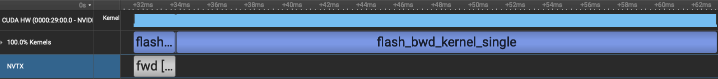
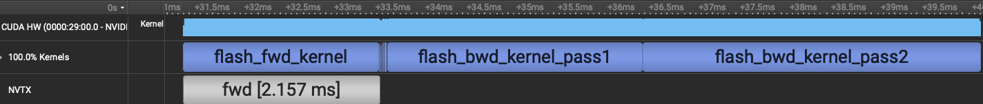
While both kernels have the same forward pass runtime ($\sim$ 2.19 ms), the single-kernel backward pass takes 28.9 ms whereas the two-kernel backward pass takes just 6.53 ms.
Comparison with PyTorch’s FA2
Let’s now do a final comparison of the forward and backward time of our two-pass kernel with the built-in FlashAttention kernel provided by PyTorch (version 2.10.0+cu128). We will switch over to bfloat16 and autotune our Triton kernels:
| Sequence length | PyTorch FA2 (ms) | Triton Impl (ms) | Triton / PyTorch |
|---|---|---|---|
| 8,192 | 2.517 | 3.351 | 1.33x |
| 16,384 | 7.749 | 12.287 | 1.59x |
| 32,768 | 31.197 | 46.403 | 1.49x |
| 65,536 | 111.403 | 185.191 | 1.66x |
We aren’t expecting to beat PyTorch’s FA algorithm since the underlying implementation is written in CUDA and has a much finer control of scheduling instructions onto the SMs. However, our own Triton implementation is now able to support much larger context lengths than either eager or compiled PyTorch and importantly, we have an understanding of the algorithm itself.
Conclusion
In this blog post, we took a look at both the forward and backward passes of FlashAttention2 while making use of tools such as Nsight and tile-based programming abstractions. We saw how tiling and recomputing the forward pass (twice!) during the backward pass gave us massive gains over a baseline PyTorch implementation. Overall, this algorithm illustrates an important point when programming GPUs which is to keep the tensor cores as busy as possible while reducing data movement, memory consumption, and atomic adds.
While we focused on FA2, both FA3 and FA4 at a high level make further use of the functional units on both Hopper and the more recent Blackwell GPUs. FA4 was also written entirely in the CuTE DSL, which I am excited to learn about and try out!
Extra
If you have any feedback or spot any errors, please feel free to reach out! I used language models to build the scaffolding for the repo (i.e., the benchmarking and testing), which rapidly sped up my development time. I wrote the Triton kernels by hand once I had a decent diagram of the algorithm.
Acknowledgements
Please check out CS336 which largely inspired this post, and thanks to Percy Liang for greenlighting the blog post!
Footnotes
-
The original FlashAttention paper. ↩
-
Horace He has an excellent blog post that touches upon data movement among other things. ↩